Ecological modeling

You will find basic R codes

1+2

[1] 3

# Load necessary library
library(deSolve)

Warning: package 'deSolve' was built under R version 4.3.3

# Define a simple Lotka-Volterra predator-prey model
lotka_volterra <- function(t, state, parameters) {
  with(as.list(c(state, parameters)), {
    dPrey <- prey * (alpha - beta * predator)
    dPredator <- predator * (delta * prey - gamma)
    list(c(dPrey, dPredator))
  })
}

# Initial state values
state <- c(prey = 40, predator = 9)

# Parameters: growth rate of prey, predation rate, reproduction rate of predator, and death rate of predator
parameters <- c(alpha = 0.1, beta = 0.02, delta = 0.01, gamma = 0.1)

# Time sequence for the simulation
time <- seq(0, 200, by = 1)

# Solve the differential equations
output <- ode(y = state, times = time, func = lotka_volterra, parms = parameters)

# Convert output to a data frame
output <- as.data.frame(output)

# Plot the results
plot(output$time, output$prey, type = "l", col = "blue", xlab = "Time", ylab = "Population", main = "Lotka-Volterra Predator-Prey Model")
lines(output$time, output$predator, col = "red")
legend("topright", legend = c("Prey", "Predator"), col = c("blue", "red"), lty = 1)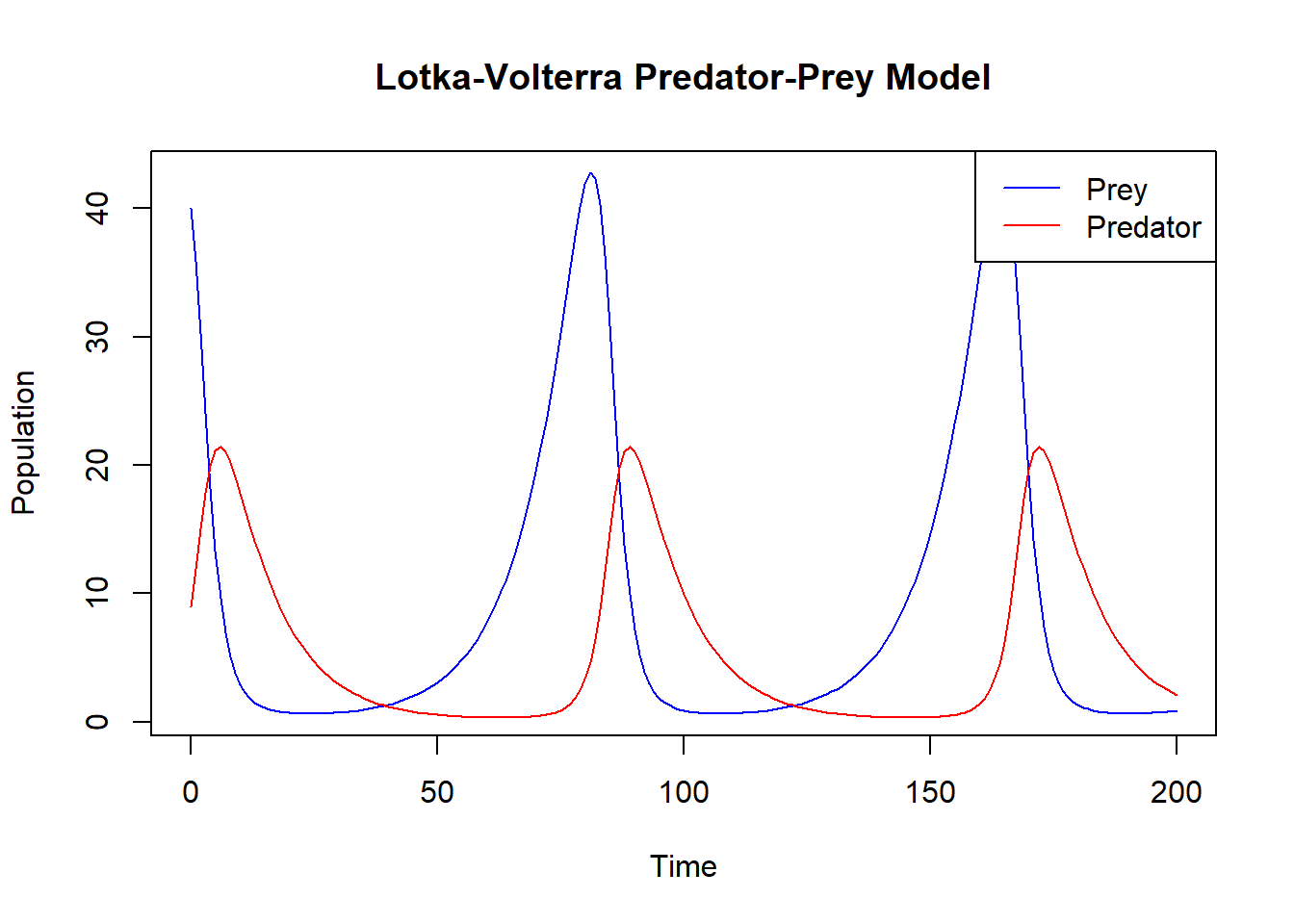

# Load necessary library
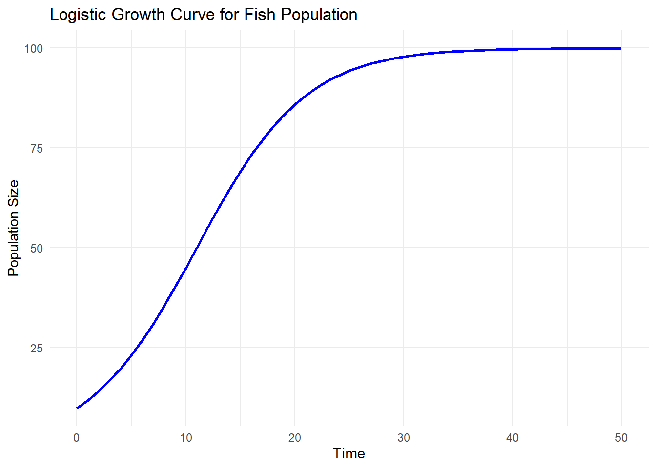
library(ggplot2)

Warning: package 'ggplot2' was built under R version 4.3.3

# Define the logistic growth function
logistic_growth <- function(t, K, r, N0) {
  K / (1 + ((K - N0) / N0) * exp(-r * t))
}

# Parameters for the logistic growth curve
K <- 100  # Carrying capacity
r <- 0.2  # Growth rate
N0 <- 10  # Initial population size

time <- seq(0, 50, by = 1)  # Time sequence

# Calculate population size over time
population <- logistic_growth(time, K, r, N0)

# Create a data frame for plotting
data <- data.frame(Time = time, Population = population)

# Plot the logistic growth curve
ggplot(data, aes(x = Time, y = Population)) +
  geom_line(color = "blue", size = 1) +
  labs(title = "Logistic Growth Curve for Fish Population",
       x = "Time",
       y = "Population Size") +
  theme_minimal()

Warning: Using `size` aesthetic for lines was deprecated in ggplot2 3.4.0.
ℹ Please use `linewidth` instead.